
Flood filling the sign of a 2D distance field with resolution 573×502 
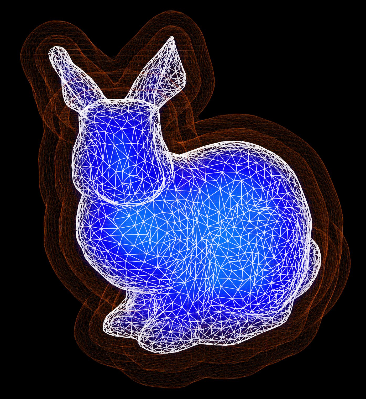
Flood filling the sign of a 3D distance field with resolution 38 x 38 x 34
Recall that even the pioneering old-school MS Paint provided its users with the famous paint bucket (fill) tool ![]() . Virtually all 2D graphics software has some variant of this tool. Given a raster image, we can fill any region with our desired color using a recursive procedure starting from the clicked pixel (seed) and checking each pixel’s neighbors whether they have the same original color as the starting pixel. All pixels with the same color as the seed pixel get re-colored to the fill color.
. Virtually all 2D graphics software has some variant of this tool. Given a raster image, we can fill any region with our desired color using a recursive procedure starting from the clicked pixel (seed) and checking each pixel’s neighbors whether they have the same original color as the starting pixel. All pixels with the same color as the seed pixel get re-colored to the fill color.
Distance fields 


This gives rise to the signed distance function defined as: 
Computing the sign of a distance field also removes the 

Continuum vs. Discrete Approach
Given a 2D curve 


The same holds for surfaces 


However, when we allow self-intersections and/or holes in the outline shape

A technique introduced by A. Baerentzen and H. Aanaes (DTU Copenhagen) relies on computing angle-weighted pseudonormals 


The technique relies on a property of surfaces (as manifolds) called orientability . Without elaborating too much on the general definition, orientability can be thought of as the possibility to define a continuous non-vanishing flow (vector field), the consequence of which is that a normal vector can be extended into the ambient space at each point. The math enthusiasts among the readers, surely heard about the Möbius strip or a Klein bottle as “shapes which only have a single side”. Although they are generally not used in most graphics applications, meshes with non-orientable manifold structure might be problematic in the sign computation even using the angle-weighted pseudonormal approach.
Although the angle-weighted pseudonormal technique extends the reach of signed distance fields to a wider variety of shapes, it presented a performance obstacle which I wanted to avoid all along. Given the previous post outlining a fast method for computing an unsigned distance field, it would make no sense to slow the computation down by processing all grid points one more time and perhaps utilizing the AABB tree for finding the closest mesh vertex. Readers who prefer this approach, however, might want to avoid constructing Octree for voxel outline and implementing the Fast Sweeping algorithm, and instead just use the AABB tree for the closest point lookup and run through the entire grid.
Due to reasons mentioned above I chose a discrete approach over a continuous one. My implementation uses the fact that the voxel outline (of sufficient resolution) encloses the (approximated) interior, and the sign function is undefined for meshes with holes.

Flood Fill Algorithm
Recall that during writing the voxel outline of the triangle mesh, we froze the outline voxels. Now even though the values of the distance function vary at each grid point, given a triangle mesh without holes the outline of frozen cells forms a closed boundary. In fact, a buffer with the same dimension as the grid values, containing binary values (0 or 1 – unfrozen, frozen), is stored. This means that we have a 3D equivalent of an image with just two colors. We can take our paint bucket tool and color all pixels/voxels inside the outline with any color we want.
As we update the frozenCells field, the distGrid field needs to be updated as well. We start by negating the entire distance grid (NegateData), i.e.: all distance values are now negative (as should be in
The preferred data structure for this is LIFO stack (in C++ std::stack) where we store pairs (or triples) of grid indices 
void ComputeSignFloodFill2D(double* distGrid, bool* frozenCells, ImageParams* imgPar)
{
	NegateData(distGrid, imgPar);

	double val; int gridPos;
	const int row = imgPar->row;
	const int nx = imgPar->width - 1;
	const int ny = imgPar->height - 1;
	int ix = 0, iy = 0;

	std::stack<std::tuple<int, int>> stack = {};
	std::tuple<int, int> idsPair;
	// find the first unfrozen cell
	gridPos = 0;
	while (frozenCells[gridPos]) {
		ix += (ix < nx ? 1 : 0);
		iy += (iy < ny ? 1 : 0);
		gridPos = row * iy + ix;
	}
	stack.push({ ix, iy });
	// a simple pixel flood
	while (stack.size()) {
		idsPair = stack.top();
		stack.pop();
		ix = std::get<0>(idsPair);
		iy = std::get<1>(idsPair);
		gridPos = row * iy + ix;
		if (!frozenCells[gridPos]) {
			val = -1.0 * distGrid[gridPos];
			distGrid[gridPos] = val;
			frozenCells[gridPos] = true; // freeze cell when done
			if (ix > 0) {
				stack.push({ ix - 1, iy });
			}
			if (ix < nx) {
				stack.push({ ix + 1, iy });
			}
			if (iy > 0) {
				stack.push({ ix, iy - 1 });
			}
			if (iy < ny) {
				stack.push({ ix, iy + 1 });
			}
		}
	}
}
Extending the above method to a 3D grid is straight-forward. Moreover, it can be sped up by processing pixels by storing and processing triples of indices 
__m128i SIMD register (with one empty int value at the end, of course).

Completing the Signed Distance Computation
A truly robust algorithm requires special mesh pre-processing to provide a closed input manifold. An alternative to pre-processing is to construct a set of angle-weighted outward-pointing pseudonormals at each mesh vertex to determine the sign function value 
ComputeSignFloodFill2D :

This is where the largest performance bottleneck comes in. Recursive grid processing of the entire grid is still, despite all optimization attempts, the most time-consuming procedure since it needs to operate on a stack container which is generally slow to work with (push, pop operations). This means that the computational load increases even faster than that of the Fast Sweeping step:

However, grids with resolution 


waiting a few seconds for larger grids does not seem like a too much of a handicap for general computational purposes (e.g. Lagrangian evolution controlled by advection field

That being said, I hope my last four posts helped those of you who sought a way to implement fast signed distance field computation generated by polygonal meshes. I am aware that this approach is far from optimal and does not use any multithreading. One could also optimize the real-time update by letting low-resolution grids render first, and then successively increasing the grid resolution up to the desired result. I put substantial emphasis on explaining the underlying theory, but if you feel like my explanations are too far off for you, feel free to leave a comment and/or contact me if you have some questions.
Happy coding!
