Eikonal Solver for the Distance Function to Triangular Meshes

I would start with a warning, that this post is going to be slightly more mathematical than the previous ones, so for the “copy-pasters” out there: feel free to skip to the code snippets which you can adjust according to your needs. If you’re not in a hurry and curious about how this method works, do read through my take on the underlying theory.
After implementing a fast enough approach to find the voxel outline of a polygonal mesh, we have everything we need to proceed to the next step of completing the distance field computation. To elaborate on the current state of our scalar grid with domain ![G = [G_{x, \min}, G_{x, \max}] \times [G_{y, \min}, G_{y, \max}] \times [G_{z, \min}, G_{z, \max}]](https://s0.wp.com/latex.php?latex=G+%3D+%5BG_%7Bx%2C+%5Cmin%7D%2C+G_%7Bx%2C+%5Cmax%7D%5D+%5Ctimes+%5BG_%7By%2C+%5Cmin%7D%2C+G_%7By%2C+%5Cmax%7D%5D++%5Ctimes+%5BG_%7Bz%2C+%5Cmin%7D%2C+G_%7Bz%2C+%5Cmax%7D%5D+&bg=000000&fg=ffffff&s=2&c=20201002)


Mathematically, the distance function: 

which is a specific case for a general n-dimensional Eikonal equation: 


The boundary condition says that the distance to an object at any of the object’s points is zero, and it increases linearly with slope 1 in the direction “away from” the source. The gradient operator 
Eikonal Solvers
Since the Eikonal equation is a non-linear hyperbolic PDE of second order, its exact solutions are hard to find. In fact, there are only a few exact solutions for the distance function equation (e.g.: the 


Hyperbolic equations describe “conservation laws“, that is, some quantity is conserved in the system’s evolution. For example the solutions to the wave equation 
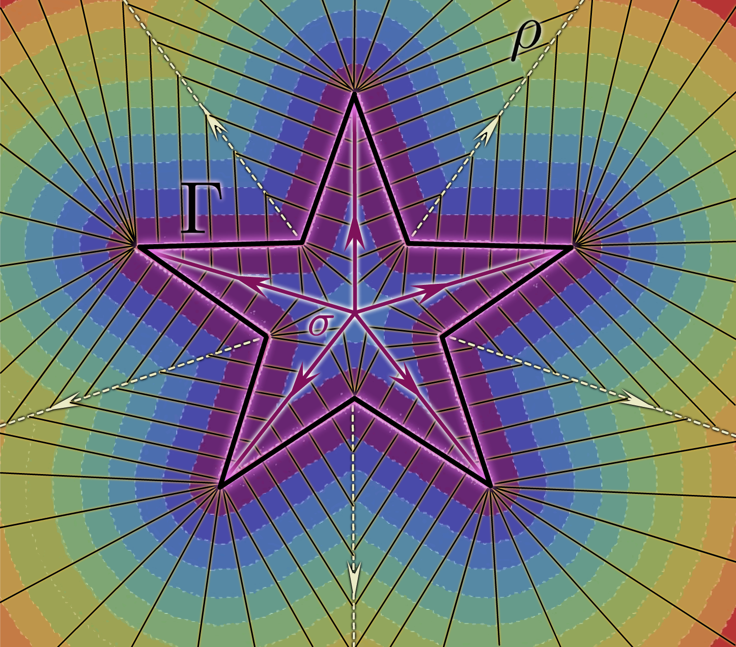
In particular, the characteristics of the Eikonal distance equation 

Characteristics cannot intersect (and for linear hyperbolic systems they follow this property) because otherwise the system of ODE’s would not have a unique solution at these intersection points. The reader then notices that for the distance function 


A contour plot of the distance function to a star-shaped outline
The property of outward propagation of information is used in algorithms computing numerical solutions to the Eikonal problem. In this section, we mention two possibilities, the latter of which will be used.

One possibility is to use the Fast Marching Method (FMM) which utilizes the same principle as Dijkstra’s algorithm, namely that the information flows outward from a given seeding area by updating the neighbor with the smallest value. The worst case complexity of the FMM is 

In a 2005 paper by Hongkai Zhao the 90’s FMM scheme by Sethian was dwarfed by the Fast Sweeping Algorithm with linear complexity 
Zhao’s Fast Sweeping Method
The input data for the Fast Sweeping Method is a domain 
DBL_MAX ). In 


A C++ implementation of the method, given a grayscale image giving rise to the input distance grid distGrid with marked outline pixels as “frozen”, and DBL_MAX everywhere else would look something like this:
void FastSweep2D(double* distGrid, bool* frozenCells, ImageParams* imgPar)
{
	const int height = imgPar->height, width = imgPar->width;
	const int row = imgPar->row;

	const int NSweeps = 4;
	// sweep directions { start, end, step }
	const int dirX[NSweeps][3] = { {0, width - 1, 1} , {width - 1, 0, -1}, {width - 1, 0, -1}, {0, width - 1, 1} };
	const int dirY[NSweeps][3] = { {0, height - 1, 1}, {0, height - 1, 1}, {height - 1, 0, -1}, {height - 1, 0, -1} };
	double aa[2], eps = 1e-6;
	double d_new, a, b;
	int s, ix, iy, gridPos;
	const double h = 1.0, f = 1.0;

	for (s = 0; s < NSweeps; s++) {

		for (iy = dirY[s][0]; dirY[s][2] * iy <= dirY[s][1]; iy += dirY[s][2]) {
			for (ix = dirX[s][0]; dirX[s][2] * ix <= dirX[s][1]; ix += dirX[s][2]) {

				gridPos = iy * row + ix;

				if (!frozenCells[gridPos]) {

					// === neighboring cells (Upwind Godunov) ===
					if (iy == 0 || iy == (height - 1)) {
						if (iy == 0) {
							aa[1] = distGrid[gridPos] < distGrid[(iy + 1) * row + ix] ? distGrid[gridPos] : distGrid[(iy + 1) * row + ix];
						}
						if (iy == (height - 1)) {
							aa[1] = distGrid[(iy - 1) * row + ix] < distGrid[gridPos] ? distGrid[(iy - 1) * row + ix] : distGrid[gridPos];
						}
					}
					else {
						aa[1] = distGrid[(iy - 1) * row + ix] < distGrid[(iy + 1) * row + ix] ? distGrid[(iy - 1) * row + ix] : distGrid[(iy + 1) * row + ix];
					}

					if (ix == 0 || ix == (width - 1)) {
						if (ix == 0) {
							aa[0] = distGrid[gridPos] < distGrid[iy * row + (ix + 1)] ? distGrid[gridPos] : distGrid[iy * row + (ix + 1)];
						}
						if (ix == (width - 1)) {
							aa[0] = distGrid[iy * row + (ix - 1)] < distGrid[gridPos] ? distGrid[iy * row + (ix - 1)] : distGrid[gridPos];
						}
					}
					else {
						aa[0] = distGrid[iy * row + (ix - 1)] < distGrid[iy * row + (ix + 1)] ? distGrid[iy * row + (ix - 1)] : distGrid[iy * row + (ix + 1)];
					}

					a = aa[0]; b = aa[1];
					d_new = (fabs(a - b) < f * h ? (a + b + sqrt(2.0 * f * f * h * h - (a - b) * (a - b))) * 0.5 : std::fminf(a, b) + f * h);

					distGrid[gridPos] = distGrid[gridPos] < d_new ? distGrid[gridPos] : d_new;
				}
			}
		}
	}
}
Drawing the result onto an image with pixel values from ![[0, 255]](https://s0.wp.com/latex.php?latex=%5B0%2C+255%5D+&bg=000000&fg=ffffff&s=2&c=20201002)
![[d_{\min}, d_{\max}]](https://s0.wp.com/latex.php?latex=%5Bd_%7B%5Cmin%7D%2C++d_%7B%5Cmax%7D%5D+&bg=000000&fg=ffffff&s=2&c=20201002)


Note that the zero-value outline was inverted to white color to be distinguishable from dark gray colors close to the outline
The specific details of each step in each sweep rely on mathematics provided by Zhao’s paper. Of course, only cells that are not frozen are processed. And only cells in 


The Godunov upwind difference scheme corresponds to a finite volume scheme (for pixels/voxels) for conservation laws (given a hyperbolic PDE) such that it is sensitive to the direction of propagation in a flow problem (along characteristics). In Zhao’s 2D formulation for a grid point 

![[(d_{i,j}^h - d_{x, \min}^h)^{+}]^2 + [(d_{i,j}^h - d_{y, \min}^h)^{+}]^2 = f_{i,j}^2 h^2](https://s0.wp.com/latex.php?latex=%5B%28d_%7Bi%2Cj%7D%5Eh+-+d_%7Bx%2C+%5Cmin%7D%5Eh%29%5E%7B%2B%7D%5D%5E2+%2B+%5B%28d_%7Bi%2Cj%7D%5Eh+-+d_%7By%2C+%5Cmin%7D%5Eh%29%5E%7B%2B%7D%5D%5E2+%3D+f_%7Bi%2Cj%7D%5E2+h%5E2+&bg=000000&fg=ffffff&s=2&c=20201002)

Where 


The individual (Gauss-Seidel) iterations look for the unique solution to a quadratic equation
![[(x-a)^{+}]^2 + [(x-b)^{+}]^2 = f_{i,j}^2 h^2](https://s0.wp.com/latex.php?latex=%5B%28x-a%29%5E%7B%2B%7D%5D%5E2+%2B+%5B%28x-b%29%5E%7B%2B%7D%5D%5E2+%3D+f_%7Bi%2Cj%7D%5E2+h%5E2+&bg=000000&fg=ffffff&s=2&c=20201002)
where 


Values of 


For reference, see line 39 of the code snippet. We use a full array of coefficients 
![[(x-a_1)^{+}]^2 + [(x-a_2)^{+}]^2 + ... + [(x-a_n)^{+}]^2= f_{i,j}^2 h^2](https://s0.wp.com/latex.php?latex=%5B%28x-a_1%29%5E%7B%2B%7D%5D%5E2+%2B+%5B%28x-a_2%29%5E%7B%2B%7D%5D%5E2+%2B+...+%2B+%5B%28x-a_n%29%5E%7B%2B%7D%5D%5E2%3D+f_%7Bi%2Cj%7D%5E2+h%5E2+&bg=000000&fg=ffffff&s=2&c=20201002)
The condition that holds for 

aa in our implementation). Then we recursively add values 


such that 

void FastSweep3D(double* grid, bool* frozenCells, GridParams* gridPar) {
   /* ... */
   /* initialization & iterating from 8 corners */

   uint gridPos = ((iz * Ny + iy) * Nx + ix);

   if (!frozenCells[gridPos]) {
    // === neighboring cells (Upwind Godunov) ...
    // ... same as for 2D image, but with all domain walls & corners ===
    // ...
        // simple bubble sort
        if (aa[0] > aa[1]) { tmp = aa[0]; aa[0] = aa[1]; aa[1] = tmp; }
        if (aa[1] > aa[2]) { tmp = aa[1]; aa[1] = aa[2]; aa[2] = tmp; }
        if (aa[0] > aa[1]) { tmp = aa[0]; aa[0] = aa[1]; aa[1] = tmp; }

        double d_curr = aa[0] + h * f; // just a linear equation with the first neighbor value
        double d_new;
        if (d_curr <= (aa[1] + eps)) {
            d_new = d_curr; // accept the solution
        }
        else {
            // quadratic equation with coefficients involving 2 neighbor values aa
            double a = 2.0;
            double b = -2.0 * (aa[0] + aa[1]);
            double c = aa[0] * aa[0] + aa[1] * aa[1] - h * h * f * f;
            double D = sqrt(b * b - 4.0 * a * c);
            // choose the minimal root
            d_curr = ((-b + D) > (-b - D) ? (-b + D) : (-b - D)) / (2.0 * a);

            if (d_curr <= (aa[2] + eps))
                d_new = d_curr; // accept the solution
            else {
                // quadratic equation with coefficients involving all 3 neighbor values aa
                a = 3.0;
                b = -2.0 * (aa[0] + aa[1] + aa[2]);
                c = aa[0] * aa[0] + aa[1] * aa[1] + aa[2] * aa[2] - h * h * f * f;
                D = sqrt(b * b - 4.0 * a * c);
                // choose the minimal root
                d_new = ((-b + D) > (-b - D) ? (-b + D) : (-b - D)) / (2.0 * a);
            }
        }
        // update if d_new is smaller
        grid[gridPos] = grid[gridPos] < d_new ? grid[gridPos] : d_new
   }

   /* for-loops scope ends */
   /* ... */
}
The grid corners with step s as triples (e.g: 


The procedure of updating field voxels according to radiating characteristics of the Eikonal problem relies on a simple geometric fact that the solution gets updated by the velocity * distance step, i.e.: 
After a closer look at the 2D algorithm’s logic applied to each voxel, we notice that if 


By sorting neighbor cell values 


The updating procedure can move against the direction of characteristics when it updates voxels with LARGE_VAL value (those that have not yet been processed). A closer look at the animation for the star image shows that during the first sweep the grid values in the interior 
The “closeness” of the 


LARGE_VAL) and balance out: 


When the same cell is re-visited in the next sweep it gets updated when it is necessary. To make sure that distance values are not biased in the direction of the last sweep, we verify whether the computed new value candidates are lower than the current cell value. If that is the case, we should, of course, consider the minimum distance value, otherwise we need to keep the old distance value. The latter should happen in the interior of

8 sweeps animation 
Complete distance field 
absError = | d_FS – d_Exact |
Final Remarks
The complete procedure for computing a distance field (without computing a sign dependent on position in 

The computation times (in seconds) on my machine for different grid resolutions and individual steps of the overall algorithm are listed in the table below:

Clearly, the demands get higher for larger grids, but the overall time is orders of magnitude better than the brute force approach. I still computed the exact distance field 


where 

To verify the computation one should compare 


In the next post I will finalize the signed distance computation by introducing an easy-to-implement method using voxel flood fill for sign computation.
