AABB Tree

A Bounding Volume Hierarchy for Computing Generic Signed Distance Fields to Mesh Objects

by Martin Cavarga

My last post ended with a problem statement: how would we generate a distance field around arbitrary mesh objects? One can easily come to a conclusion that the vast majority of objects used in 3D modeling are not geometric primitives or their Boolean combinations. In practice, we can easily start with a point-cloud model (perhaps from a 3D scan or photogrammetry) upon which a triangulation algorithm is applied. Having no other information than a vertex array and connectivity information (vertex indices) we need to sample the space surrounding this mesh object so that each sampling point locates the closest mesh triangle and computes a point-to-triangle distance.

The easiest way to approach this problem is to “brute-force” the computation for the entire mesh:

void Grid::BruteForceDistanceField(Geometry* geom)
{
	int ix, iy, iz, i, gridPos;
	Vector3 p = Vector3(); Tri T;

	Vector3 o = m_BBox.min; // origin
	uint nx = m_Nx - 1;
	uint ny = m_Ny - 1;
	uint nz = m_Nz - 1;
	double dx = m_Scale.x / nx;
	double dy = m_Scale.y / ny;
	double dz = m_Scale.z / nz;
	double result_distSq, distSq;

	for (iz = 0; iz < m_Nz; iz++) {
		for (iy = 0; iy < m_Ny; iy++) {
			for (ix = 0; ix < m_Nx; ix++) {

				result_distSq = DBL_MAX;
				p.set(
					o.x + ix * dx,
					o.y + iy * dy,
					o.z + iz * dz
				);

				for (i = 0; i < geom->vertexIndices.size(); i += 3) {
					T[0] = &geom->uniqueVertices[geom->vertexIndices[i]];
					T[1] = &geom->uniqueVertices[geom->vertexIndices[i + 1]];
					T[2] = &geom->uniqueVertices[geom->vertexIndices[i + 2]];
					distSq = GetDistanceToATriangleSq(t, &p);

					result_distSq = distSq < result_distSq ? distSq : result_distSq;
				}

				gridPos = m_Nx * m_Ny * iz + m_Nx * iy + ix;
				m_Field[gridPos] = sqrt(result_distSq);
			}
		}
	}
}

The above (C++) method belongs to a Grid object (note that we use using uint = unsigned int for shorter identifiers). As we can see: it needs to run across the entire scalar grid (all sampling points) and for each point also accross all mesh triangles (vertexIndices with stride = 3). Lines 31 and 34 present the largest bottleneck – a triangle distance function with many conditions, and a single ternary condition updating the squared distance value result_distSq whenever a closer triangle is encountered. These two commands might not seem like much on their own, but when perfomed $N_x \times N_y \times N_z \times N_{\Delta}$ – times sequentially ( $N_{\Delta}$ is the number of triangles in the target mesh), it can get really slow. Furthermore, the computational time increases with $\mathcal{O}(M \ N_{\Delta} )$ where $M = N_x \times N_y \times N_z$ is the scalar grid’s resolution.

In fact, meshes with $N_{\Delta} \geq 5000$ and grid resolution $M = 45^3$ take over 10 minutes in Release and over 25 minutes in Debug configuration! That is nearly useless for any practical purposes, especially for a “Meta-Object” plugin with an underlying scalar field that needs to be updated in real time. With that in mind, we need a more robust approach.

When a sampling point is located near some part of a mesh, it is utterly useless to compute distances to triangles that are “on the other side” of the mesh. One might think that the concept of “closeness” to some triangles of the mesh is inseparable from the distance we intend to compute, but it turns out that there is another set of approaches utilizing a “friend” of programmers who want to accelerate a process handling arbitrarily large amounts of data – a binary tree.

Bounding Boxes and Binary Space Partitioning

An axis-aligned bounding box is an object described by two points $\textbf{b}_{\text{min}}$ and $\textbf{b}_{\text{max}}$ – the minimum and maximum corner of a box region of space respectively. This is why it is often referred to as a “min-max”. A three.js implementation of this object contains almost all necessary functionality. The only exceptions are some methods implemented and used in my version.

3D regions can be partitioned into oriented bounding boxes as well. These are oriented in space so that they fit the geometric data they contain (points, lines, triangles, primitives…). However, their construction requires some additional preprocessing, which would slow down the development of a fully functional distance field generator. Axis-aligned min-max boxes provide a cheap way to compute intersections between them and primitive data (points, lines, triangles…), and are easy to construct.

In order to compute a bounding box of an arbitrary mesh object, we just need the vertex information, in particular: traversing the vertex array and incrementing/decrementing default minimum and maximum values for each vertex coordinate. Taking a 1000 triangles we need to perform 3000 min-max operations (at worst) for each vertex, and this amount increases linearly with more data. We need to perform this only once to obtain the bounding box of our mesh geometry.

Similarly to how search engines compose search queries based on the degree of matching to the searched string, we can utilize the computationally cheap process of “localizing” geometric primitives in a hierarchy of bounding boxes. Introducing: binary space partitioning.

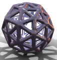
Regardless of whether we use axis-aligned bounding boxes (AABB’s) or other volume units as nodes, the fundamental idea is to start with a root node represented by the largest available bounding volume, and splitting it into two sub-volumes in each recursive step. As we can see in the above image: nodes can contain triangles (or possibly different primitives: edges, points, etc.). However, whenever a node contains primitives, it is by definition a leaf node (i.e.: at the bottom of the tree, e.g.: nodes $N_4, N_5, N_6$ and $N_7$ in the image above). It should be noted that there is no requirement for any connectivity information of individual primitives (triangles). The raw data is to be considered as separate unorganized units (e.g.: “triangle soup“).

Let us consider the computational costs of:

constructing a search tree – To create a tree one has to insert $n$ elements (primitives). The insertion cost is on average: $\mathcal{O}(\log{n})$ to worst case: $\mathcal{O}(n)$ meaning that average construction cost is $\mathcal{O}(n\log{n})$ and worst case is $\mathcal{O}(n^2)$ (all primitives clumped together at one position).
searching for the first matching result – The resulting tree can be degenerate, i.e.: a linked list with all primitives contained in the single leaf node at the end. This makes the worst case for searching $\mathcal{O}(n)$ . Most (useful) mesh geometries wouldn’t produce such case, so the search cost is only proportional to the tree height, namely: $\mathcal{O}(\log{n})$ .

Balancing the resulting tree or implementing it as self-balancing can minimize tree height, making search queries faster. Since we intend to use this tree only once, node deletion operation is not necessary. We can summarize the above costs in the following table:

The total cost for finding the closest triangle to a given point is fully described by the last row in the above table.

The remaining question is: how to partition bounding volumes every time they are to be split?

Leaf Conditions

The implications of binary space partitioning are that the workload of mesh primitives (triangles) is significantly decreased. Only the relevant (closest) triangles are considered. However, given the amount of configurations a polygon soup can be found in, the situation can easily devolve into a scenario close to the worst case if we split bounding volumes arbitrarily. Another important condition is the stopping criterion, i.e.: when to stop splitting.

We can denote the conditions under which an AABB node is no longer allowed to be split as “leaf conditions“. In my implementation they are summarized by the following inequality

$N_L + N_R < \frac{3}{2} N_{\text{total}}$

which quantifies the balance between the number of left node triangles $N_L$ with the right node triangles $N_R$ and the total number of triangles $N_{\text{total}}$ . Considering that since triangles can “share boxes”, in general: $N_L + N_R \geq N_{\text{total}}$ .

The search for the optimal split position is the largest bottleneck for the tree’s construction. The axis-aligned splitting direction should adapt to the distribution of primitives within each box, so for splitting direction we choose the longest split axis for each node splitting step. Splitting the node’s bounding box in half would be insufficient for meshes with large concentrations of primitives (triangles) in some areas since it would take longer for nodes to reach leaf conditions. And when nodes reach leaf conditions, the search query would need to handle nearly all triangles of the triangle soup when it reaches such “problematic” leaf node.

We can use a variant of a technique called surface area heuristic (SAH) which minimizes a cost function:

$f_{\text{cost}}(x) = C_L(x) \frac{SA_L(x)}{SA} + C_R(x) \frac{SA_R(x)}{SA}$

where $SA$ is the surface area of current node’s bounding box, $SA_L(x)$ and $SA_R(x)$ are surface areas of the potential left and right child node’s bounding boxes respectively (variable with respect to split position $x$ ), and cost weights $C_L(x)$ and $C_R(x)$ which evaluate the cost of traversing the left and right node candidates respectively. The traversing cost functions $C_L$ and $C_R$ are evaluated by counting primitives intersected by the left and right box candidates. Clearly, $C_L$ is non-decreasing with respect to $x$ , since by moving the split position further to the right can result in no change or more triangles contained in the left node, and $C_R$ is non-increasing for the same reason.

The cost function $f_{\text{cost}}$ is, of course, discontinuous at split positions $x$ where triangle counts are incremented/decremented and its domain $[b_{\min}, b_{\max}]$ needs to be sampled very roughly to save time. Uniform sampling of interval $[b_{\min}, b_{\max}]$ is the simplest solution to the sampling problem, but the approximation of the minimum value will be improved by adaptive resampling.

Adaptively resampled optimal split position for the first splitting of the bounding box of the Stanford Bunny model as an approximated minimum of $f_{\text{cost}}$

On most modern machines, the adaptive resampling approach allows for parallel processing of multiple split positions using 32-bit (or even 64-bit for some machines) SIMD registers.

Node Splitting

The resulting recursive node-splitting algorithm can be summarized with pseudocode as:

To account for floating point errors, each bounding box $\mathcal{B}_0$ is inflated by a small number $\varepsilon > 0$ so that triangle-box intersection subroutines do not fail. My specific C++ implementation is handled by the following Construct method:

void AABBNode::Construct(std::vector<uint>* primitiveIds, uint depthLeft)
{
	if (depthLeft == 0 || primitiveIds->size() <= 2) {
		m_PrimitiveIds = *primitiveIds;
		FilterPrimitives();
		return;
	}

	// choosing the longest split axis seems to be faster
	if ((m_BBox.max.x - m_BBox.min.x) > (m_BBox.max.y - m_BBox.min.y) && (m_BBox.max.x - m_BBox.min.x) > (m_BBox.max.z - m_BBox.min.z)) {
		m_Axis = 0;
	}
	else if ((m_BBox.max.y - m_BBox.min.y) > (m_BBox.max.z - m_BBox.min.z)) {
		m_Axis = 1;
	}
	else {
		m_Axis = 2;
	}

	std::vector<uint> leftPrimitiveIds = {};
	std::vector<uint> rightPrimitiveIds = {};
        
    // classify this node's primitives (which should go to the left and right child) & find split position
	m_SplitPosition = GetSplitPosition(*primitiveIds, &leftPrimitiveIds, &rightPrimitiveIds);

	const bool stopBranching = !HasEnoughBranching(leftPrimitiveIds.size(), rightPrimitiveIds.size(), primitiveIds->size());
	if (stopBranching) {
		m_PrimitiveIds = *primitiveIds;
		FilterPrimitives();
	}
	else {
		if (leftPrimitiveIds.size() > 0) {
			Box3 bboxLeft = m_BBox;
			bboxLeft.max.SetCoordById(m_SplitPosition, m_Axis);
			m_Left = new AABBNode(&leftPrimitiveIds, bboxLeft, m_Tree, depthLeft - 1, this);

			if (m_Left->m_PrimitiveIds.empty() && m_Left->m_Left == nullptr && m_Left->m_Right == nullptr) {
				m_Left = nullptr;
			}
		}
		if (rightPrimitiveIds.size() > 0) {
			Box3 bboxRight = m_BBox;
			bboxRight.min.SetCoordById(m_SplitPosition, m_Axis);
			m_Right = new AABBNode(&rightPrimitiveIds, bboxRight, m_Tree, depthLeft - 1, this);

			if (m_Right->m_PrimitiveIds.empty() && m_Right->m_Left == nullptr && m_Right->m_Right == nullptr) {
				m_Right = nullptr;
			}
		}
	}
}

Implemented for AABBNode struct:

struct AABBNode {
   AABBNode* m_Parent = nullptr;
   AABBNode* m_Left = nullptr;
   AABBNode* m_Right = nullptr;
   // ptr to an object containing the root AABBNode and raw primitives (triangles, edges, vertices)
   AABBTree* m_Tree = nullptr;

   Box3 m_BBox;
   std::vector<uint> m_PrimitiveIds = {};
   uint m_Axis = 2; // (X, Y, Z) -> (0, 1, 2)
   float m_SplitPosition = 0.0f; 
   
   // constructor
   AABBNode(std::vector<uint>* primitiveIds, Box3& bbox, AABBTree* tree, uint depthLeft = MAX_DEPTH, AABBNode* parent = nullptr);
   
   // filters only primitives which actually intersect m_BBox
   void FilterPrimitives();
   // classifies this node's primitives (which should go to the left and right child) & returns (optimal) split position
   float GetSplitPosition(std::vector<uint>& primitiveIds, std::vector<uint>* out_left, std::vector<uint>* out_right);
   // returns true if this node has no children
   bool IsALeaf();
   // returns true if this node contains primitive ids and has no children
   bool IsALeafWithPrimitives();
};

// leaf condition for AABBNode
bool HasEnoughBranching(size_t nLeftPrims, size_t nRightPrims, size_t nPrims) {
    return nLeftPrims + nRightPrims < 1.5f * nPrims;
}

The implementation of GetSplitPosition method can be user-controlled or chosen automatically between a version which uses SIMD registers and a purely sequential version.

The m_PrimitiveIds array contains indices to primitives (triangles, edges, or vertices) so they do not need to be copied with their coordinates for each node. Aside from the root AABBNode, the tree object m_Tree contains raw primitives indexed by m_PrimitiveIds.

Intersection and Distance Queries

By implementing the above tree, we are free to proceed to the next step: implementing desired search queries. The two obvious candidates are:

box-primitive intersection
closest primitive to a point

These will need to be implemented in the tree object AABBTree (a pointer to which is stored in each AABBNode as m_Tree). The first query can be carried out via method:

bool AABBTree::BoxIntersectsAPrimitive(Box3* box)
{
	std::stack<AABBNode*> stack = {};
	stack.push(m_Root);
	AABBNode* item;
	Vector3 center; Vector3 halfSize;
	box->setToCenter(&center); // writes box center to center
	box->setToHalfSize(&halfSize); // writes box half-size to halfSize

	while (stack.size()) {
		item = stack.top();
		stack.pop();

		if (item->IsALeaf()) {
			for (auto pId : item->m_PrimitiveIds) {
				if (GetPrimitiveBoxIntersection(m_Primitives.at(pId), &center, &box->min, &box->max, &halfSize, 0.0f)) {
					return true;
				}
			}
		}
		else {
			if (item->m_Left && box->intersectsBox(item->m_Left->m_BBox)) {
				stack.push(item->m_Left);
			}
			if (item->m_Right && box->intersectsBox(item->m_Right->m_BBox)) {
				stack.push(item->m_Right);
			}
		}
	}

	return false;
}

where GetPrimitiveBoxIntersection is specifically handled for each type of primitive:

bool GetPrimitiveBoxIntersection(Primitive& primitive, Vector3* boxCenter, Vector3* boxMin, Vector3* boxMax, Vector3* boxHalfSize, double offset)
{
	if (primitive.vertices.size() == 1) {
		return (
			(primitive.vertices[0]->x >= boxMin->x && primitive.vertices[0]->x <= boxMax->x) &&
			(primitive.vertices[0]->y >= boxMin->y && primitive.vertices[0]->y <= boxMax->y) &&
			(primitive.vertices[0]->z >= boxMin->z && primitive.vertices[0]->z <= boxMax->z)
		);
	}
	else if (primitive.vertices.size() == 2) {
		return GetEdgeBoxIntersection(primitive.vertices, boxMin, boxMax);
	}
	else if (primitive.vertices.size() == 3) {
		Tri t = new Vector3*[3];
		t[0] = primitive.vertices[0];
		t[1] = primitive.vertices[1];
		t[2] = primitive.vertices[2];
		return GetTriangleBoxIntersection(t, boxCenter, boxHalfSize);
		delete[] t;
	}

	return false;
}

A better way of implementing this method would be to pass it as a lambda expression into BoxIntersectsAPrimitive with implementation specific for the primitive type. The GetEdgeBoxIntersection and GetTriangleBoxIntersection methods have been optimized and are inspired by multiple sources.

The AABBTree object can be used for distance queries as well, for example:

AABBNode* AABBTree::GetClosestLeafNode(Vector3& point)
{
	std::stack<AABBNode*> stack = {};
	stack.push(m_Root);
	AABBNode* item; AABBNode* nearNode; AABBNode* farNode;
	bool leftIsNear;

	while (stack.size()) {
		item = stack.top();
		stack.pop();

		if (item->IsALeaf()) {
                    return item;
		}
		else {
			leftIsNear = point.getCoordById(item->m_Axis) < item->m_SplitPosition;
			nearNode = item->m_Left;
			farNode = item->m_Right;
			if (!leftIsNear) {
				nearNode = item->m_Right;
				farNode = item->m_Left;
			}

			if (nearNode) {
				stack.push(nearNode);
			}
			else if (farNode) {
				stack.push(farNode);
			}
		}
	}

	return nullptr;
}

The closest leaf node can then provide a small number of primitives which can easily be compared for distance.

A modification of BoxIntersectsAPrimitive is a method that returns all primitives in a box:

void AABBTree::GetPrimitivesInABox(Box3* box, std::vector<uint>* primIdBuffer)
{
	if (!primIdBuffer->empty()) primIdBuffer->clear();

	std::stack<AABBNode*> stack = {};
	stack.push(m_Root);
	AABBNode* item;

	while (stack.size()) {
		item = stack.top();
		stack.pop();

		if (item->IsALeaf()) {
			for (auto pId : item->m_PrimitiveIds) {
				primIdBuffer->push_back(pId);
			}
		} else {
			if (item->m_Left && box->intersectsBox(item->m_Left->m_BBox)) {
				stack.push(item->m_Left);
			}
			if (item->m_Right && box->intersectsBox(item->m_Right->m_BBox)) {
				stack.push(item->m_Right);
			}
		}
	}
}

The average complexity of GetPrimitivesInABox is $\mathcal{O}(\log{n})$ since the number of steps till a leaf node is reached is proportional to the depth of AABBTree. The same holds for GetClosestLeafNode even though measured times may differ due to specific operations.

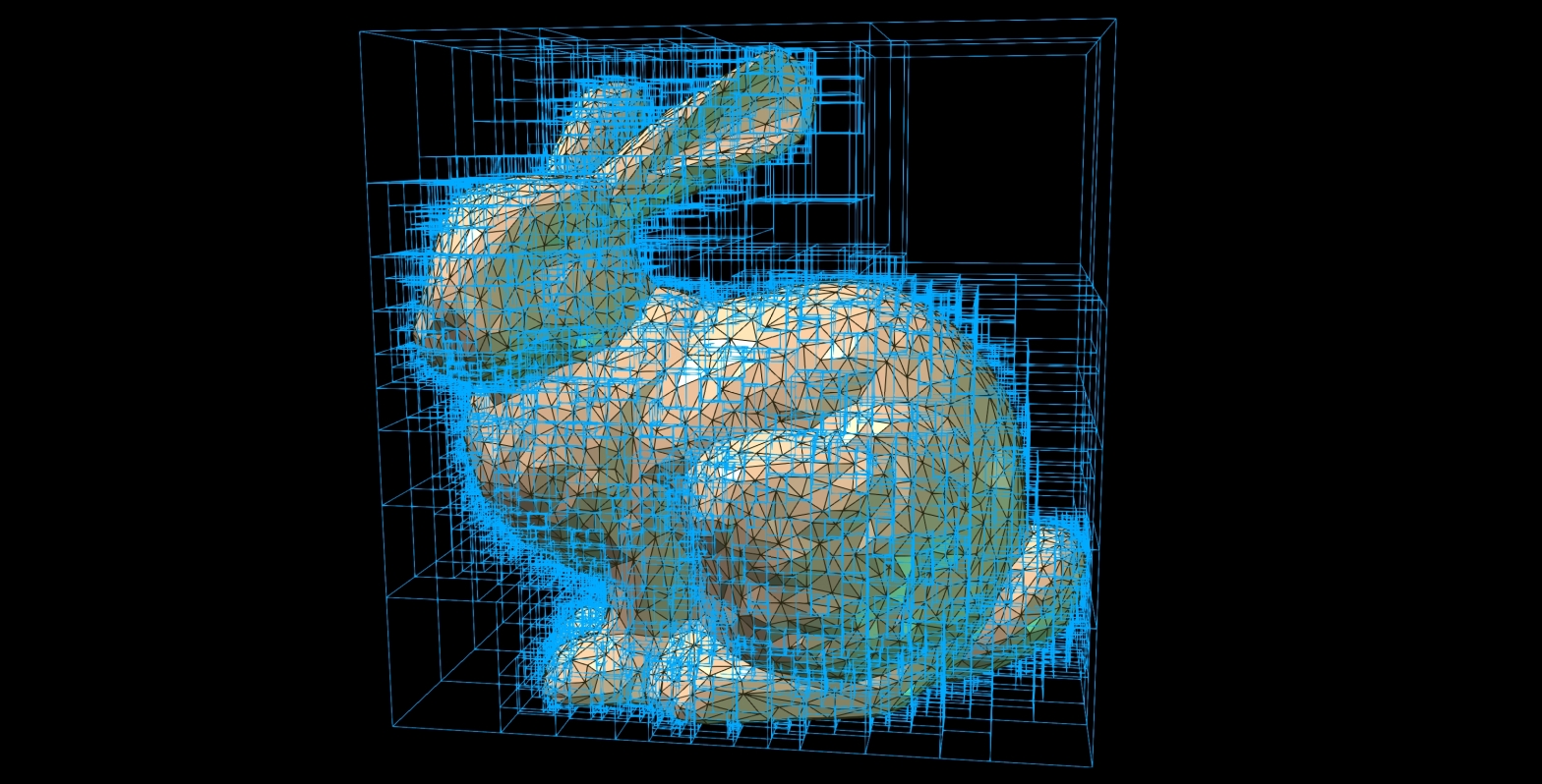
A visual representation of `AABBNode` bounding boxes, with (left) all nodes, and (right) just leaf nodes.

Animation showing leaf nodes with their triangles for each level of tree depth.

Final Remarks

The construction of AABBTree object for the Stanford Bunny model takes, on average, 0.05 seconds on my machine. However, this implementation has no balancing or additional optimization (besides using SIMD registers). Still compared to other subroutines used in my implementation of an SDF generator the construction of AABBTree takes only about 4% of computation time for scalar grid resolution $100^3$ .

The resulting AABBTree is later used for accelerated intersection query with BoxIntersectsAPrimitive and obtaining relevant (close) primitives via GetPrimitivesInABox. These methods will later be used when constructing an Octree object refined at volume nodes intersecting the mesh geometry.

All things considered, I chose my own implementation specific to SDF computation rather than a working implementation with a lot of functionality I wouldn’t use (e.g.: CGAL). This means that the overall design was meant for academic purposes, and is still likely very flawed, requiring additional iterations for improvement. However, I believe that this article may guide researching developers who are new to the underlying procedures of collision detection and accelerated distance querying.

Manual Birklid on Octree for Voxel Outlines of a Triangular MeshSeptember 30, 2021
very nice publish, i definitely love this website, keep on it
Nikolka Harantová on On the New Meaning of Life: Part IIAugust 27, 2021
Oooo, velmi dobre ! Dňa pi 27. 8. 2021, 16:50 Martin Cavarga napísal(a): > mshgrid posted: ” A Possible Resolution…

AABB Tree

A Bounding Volume Hierarchy for Computing Generic Signed Distance Fields to Mesh Objects

Bounding Boxes and Binary Space Partitioning

Leaf Conditions

Node Splitting

Intersection and Distance Queries

Final Remarks

Leave a comment

Cancel reply

operation	best case	average	worst case
insert a leaf node containing $n \geq 1$ elements	$\mathcal{O}(1)$	$\mathcal{O}(\log{n})$	$\mathcal{O}(n)$
insert (a necessary amount of) leaf nodes containing $n$ elements (full tree construction)	$\mathcal{O}(n)$	$\mathcal{O}(n\log{n})$	$\mathcal{O}(n^2)$
search for an element contained in a leaf node with $n \geq 1$ elements	$\mathcal{O}(1)$	$\mathcal{O}(\log{n})$	$\mathcal{O}(n)$

A Bounding Volume Hierarchy for Computing Generic Signed Distance Fields to Mesh Objects

Bounding Boxes and Binary Space Partitioning

Leaf Conditions

Node Splitting

Intersection and Distance Queries

Final Remarks

Share this:

Related

Leave a comment

Cancel reply